Developing a Basketball Minimap for Player Tracking using Broadcast Data and Applied Homography

If you’ve ever watched an ESPN video recently on Steph Curry, the analysts will typically mention how Curry has immense stamina because he ran, say 2.7 miles on the court in last night’s win. How do these analysts know exactly how much a player has moved on the court? There are a couple reasons. First, the NBA has started to place player tracking devices from third party sources, such as Kinexon. These devices track live three dimensional coordinates that represent the player’s position relative to the viewer. The second way is that the NBA sets up cameras capturing multiple views of the court and use a concept called Homography and Player Detection to capture player movement on a court. Player Tracking has become a big phenomenon in sports as it allows data scientists to make more in-depth analysis on a player’s impact based on how the player moves around the court.
For instance, teams can merge play-by-play data and player tracking simulations to add context to a player’s impact when on the court. Now, if you take a player like Draymond Green you can visualize his ability to clog up cutting lanes, get out in transition, and set effective screens. These simulations can be much easier to visualize on a two-dimensional level compared to actual game film where broadcast angles can’t capture spacing on the court as effectively. This research project is focused on exploring applications of homography on broadcast footage of basketball games from YouTube to create a two-dimensional simulated minimap.
What is Homography? A homography is a type of transformation in that we take advantage of projections to relate two images. In essence, a homography is a transformation between two images of the same scene, but from a different perspective. While the NBA captures images from numerous different locations to pinpoint a player on the court, many high school games and some collegiate games are only captured from a broadcast view. Thus, I wanted to explore the effectiveness of applying homography on broadcast footage to track player movement on the court. This could be utilized to measure distance traveled amongst certain players as well as help coaches and team faculty break down film more easily by using a 2D simulation concurrently with actual game footage.
In order to track players I needed some specific python libraries and packages to be installed. This project utilizes pytorch and the COCO dataset. PyTorch is a widely used deep learning library used for object detection. PyTorch runs detectron2 which is an open-source object detection algorithm built by Facebook (Meta). I trained it on the COCO dataset that has a set of objects that are pre-processed and recognizable by the object detection algorithm. When I apply the detectron2 visualizer on one of the initial frames from an NBA game I get the image below.
Now that detectron2 can detect both the ball and the players, I needed to reduce the noise by only capturing players that are within the court. The next step was to draw visual boundaries on our image and map it onto a 2D basketball court that will be used for our minimap. The idea is to apply the object detection within the boundaries of the court so that I am only tracking legitimate players and not fans, coaches, or referees on the sideline. The source points that represent the corners of the court will map onto the destination points that represent the corners of the 2D court image displayed below.
To understand this function, let’s refer to the picture of the card to the left. The card is displayed on a 3 dimensional level, but I am utilizing homography to transform it on a 2D plane. The lines that connect both of the source and destination points are represented as vectors. These are the vectors that are getting refactored.
From here I applied the homography function onto a set of points to convert a 3D vector into a 2D array representing a position within this specified zone on the court image. The apply homography function is shown below.
The detectron2 algorithm utilizes a DefaultPredictor.predictor method to return a list of prediction boxes of each identified object. The object classes are stored in prediction classes, where person objects are marked as 0 while a ball is marked as 32. For each predicted object that is a player or a ball, I stored the dimensions of the prediction box in a dictionary along with the transformed data point that represents the position of the player. The dictionary is then passed onto another function to create separate images around all the captured players based on the dimensions of the prediction boxes. Here is an example output of the images captured.
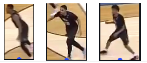
When I was initially developing the pipeline, I wanted to use the player images to capture and evaluate a sample of image pixels from the jersey to to classify the players as the home team or away team. However, what I came to notice was that Youtube broadcast data doesn’t have great resolution and moreover, when a frame is captured in the span of a player moving his body the pixels captured aren’t very clean. This led to issues in the player classification phase which led me to focus on individual player tracking with a defined set of players.
One major issue with using only broadcast data is that when players collectively move to another side of the court, the single camera is now moving and the dimensions of the homography change. Thus, I had to create three separate homography transformation algorithms that encapsulate the whole court. I hard-coded the frames within the input video in which the correct homography transformation function should be used. The three transformations are shown below.
As you can see our functions take in each frame as an image and uses OpenCV, a huge open-source library for computer vision, machine learning, and image processing, to transform the vectors of the source points onto the 2D court image shown earlier.
Once the images are captured along with their 2D player position, the next step is to add a couple more constraints to reduce noise from our output video. While I use Shapely, a python package for analyzing planar geometric objects, to check if a player object is within the court, it still may pick up fans who are sitting along the sideline, because having only one camera angle makes it difficult to draw geometric boundaries around the court. Take this frame as an example to see the amount of “noise” that is picked up. The blue dots represent players that are supposedly on the court.
Thresholds are established on the player coordinates to double check that they are truly within the courts boundaries. Once I reduced the noise, I chose a specific frame early into the input video to capture the initial players on the court and store them. This part is necessary as I do not have access to player tracking devices so I need to manually reference each player initially.
Once the initial players and their initial positions are stored, I continue to grab each frame from the input video and feed it through the data pipeline to store the set of new positions. I call a function to find the closest player to each of the individual players I have. The original hash table with the player positions are replaced with the new closest position and the players are drawn onto the 2D court image along with a line connecting the initial and new positions. The temporary list of positions collected are now reset and will capture positions for another 3 frames before passing into the find_closest_player function.
OpenCV uses a video writer to write each of these altered frames and once the video is processed fully the video writer will close and the basketball minimap is complete. The completed minimap output is shown below. OpenCV is fairly intuitive and allows the developer to set the frames-per-second speed to increase or decrease the speed. I set my video to 6 fps, so that the player movement is very easy to see. Here is the input and minimap output:
The best way to improve this project is to get better quality images around the captured players. Once this is implemented, the RGB pixel evaluation will yield more accurate results and classify the correct number of home and away players. This would improve the accuracy of the player tracking, because I can differentiate between home and away players rather than just which player is the closest to the original player’s position.
Another aspect that could be researched further is how to detect when the video should switch between the left, right, and middle boundaries. As of right now, I am manually inputting which frames to switch the homography transformation algorithm. But with improved detection capabilities, it could be possible to detect when most of the players are on a different boundary on the court and then automatically switch planar states. This would fully automate the pipeline and allow us to not hardcode the initial positions in.
Note: For more information on the full implementation of this project please visit the GitHub link below. Feel free to reach out to me through LinkedIn if you want to connect or collaborate.
